Mangrove Deforestation Analysis — Ambanja & Ambaro Bays, Madagascar

📍 Madagascar · 📅 November 2025

Tools: Python · ArcPy · Google Earth Engine

Which communities are losing the most mangrove forest — and does proximity to human infrastructure explain it? In Madagascar’s Ambanja and Ambaro Bays, a Python-based spatial pipeline built the answer from the ground up.

The Problem

One of the world’s most productive ecosystems — vanishing fast

Mangrove forests store extraordinary amounts of carbon, protect coastlines from storm surges, and sustain the livelihoods of coastal communities. In Madagascar, they are under pressure from timber harvesting, agricultural expansion, and aquaculture — driven by population growth and limited governance.

This project quantifies mangrove loss between 1999 and 2019 at two administrative scales — commune and fokontany — and tests whether proximity to paths and permanent rivers explains spatial patterns of deforestation.

The Data

A global dataset, downloaded from Google Earth Engine

The Murray Global Tidal Wetland Change dataset (Murray et al. 2022) maps tidal wetland gain and loss globally using over 1 million Landsat images combined with machine learning. It was downloaded for this project via a Google Earth Engine script, with NA values encoded as 0 in the raster.

Administrative boundaries — communes and fokontany — and infrastructure layers including paths and permanent rivers were sourced from the AAB geodatabase.

Step 1 — Pre-Processing

Converting pixels to polygons — and cleaning the noise

The Murray raster encodes mangrove loss year as pixel values, with 0 representing no data. The first task was converting it to polygon format for vector-based spatial analysis, then using ArcPy cursors to remove null records and rename the gridcode field to loss_year.

arcpy.conversion.RasterToPolygon(
    original, opath,
    "NO_SIMPLIFY",
    raster_field = 'Value'
)

# Rename gridcode to loss_year
arcpy.management.AlterField(mangrove_polygon_name, 'gridcode', 'loss_year')

# Remove null polygons using UpdateCursor
with arcpy.da.UpdateCursor(mangrove_polygon_name, 'loss_year') as cursor:
    for row in cursor:
        if row[0] == 0:
            cursor.deleteRow()

Step 2 — Loss by Commune

Where is deforestation most severe?

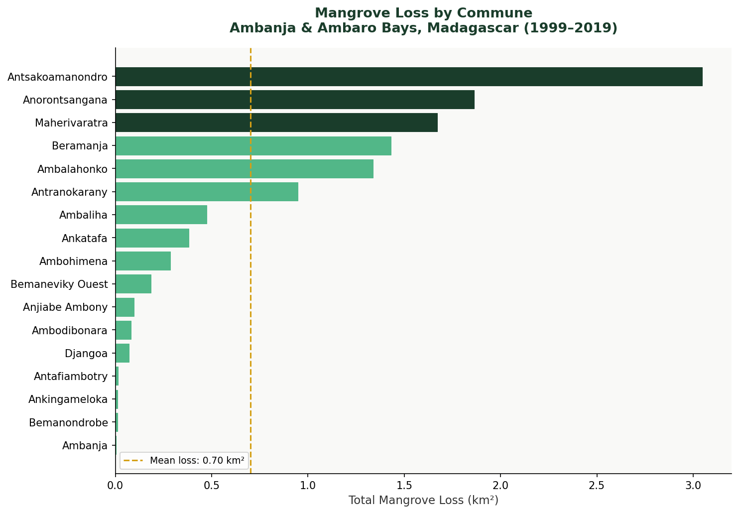
The cleaned polygons were spatially joined to commune boundaries. Area was calculated using CalculateGeometryAttributes(), then summarized with arcpy.analysis.Statistics() — grouping by commune to produce total loss area (km²) and average loss year.

arcpy.analysis.Statistics(
    in_table = joined_layer,
    out_table = summary_table,
    statistics_fields = [["Shape_Area", "SUM"], ["loss_year", "MEAN"]],
    case_field = "COMMUNE"
)

Total mangrove loss (km²) by commune, 1999–2019. Antsakoamanondro recorded the highest loss at 3.05 km², followed by Anorontsangana (1.86 km²) and Maherivaratra (1.67 km²). Dashed line shows the mean loss across all communes.

Step 3 — Fokontany Scale

Zooming in: sub-commune hotspots

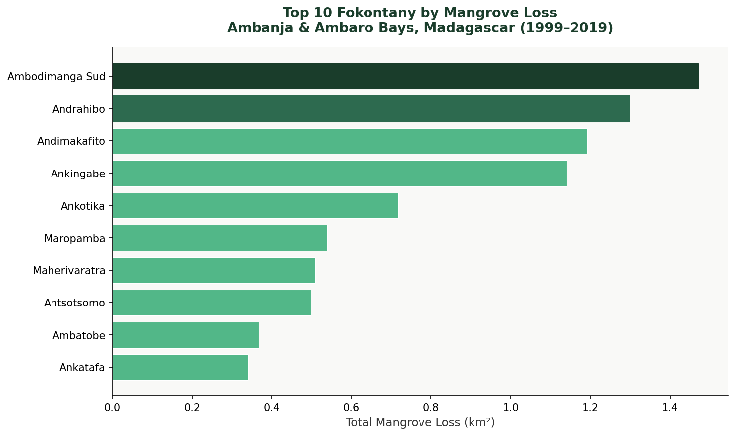
The same workflow was repeated at the fokontany level — a finer administrative unit — revealing deforestation hotspots that commune-level analysis would mask.

Top 10 fokontany by total mangrove loss. Ambodimanga Sud (1.47 km²) and Andrahibo (1.30 km²) led at the sub-commune scale.

Step 4 — Temporal Trend

When did deforestation peak?

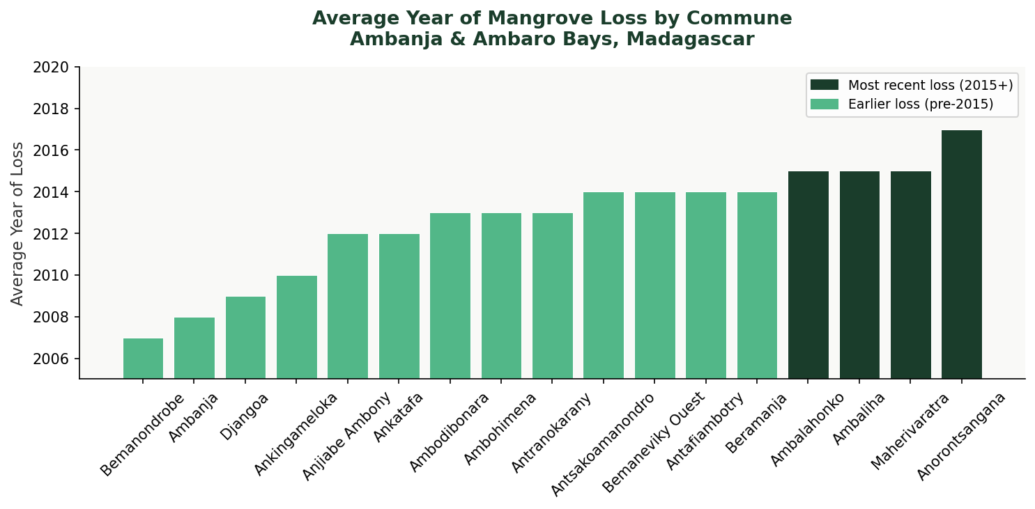
A histogram of loss year revealed that mangrove loss increased steadily until peaking around 2016, with a slight decline afterward. The map of average loss year by commune shows most deforestation concentrated between 2012 and 2015.

Average year of mangrove loss by commune. Darker bars indicate more recent deforestation events (2015 and later).

Step 5 — Proximity Analysis

Does accessibility drive deforestation?

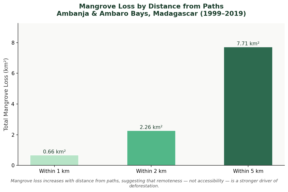
Multi-ring buffers of 1 km, 2 km, and 5 km were applied around paths and permanent rivers, then intersected with mangrove loss polygons to quantify deforestation within each distance band.

arcpy.analysis.Buffer(
    in_features = paths_layer,
    out_feature_class = buffer_output,
    buffer_distance_or_field = "1000 Meters",
    dissolve_option = "ALL"
)

arcpy.analysis.Intersect(
    in_features = [buffer_output, mangrove_polygon_name],
    out_feature_class = intersect_output
)

Total mangrove loss by distance from paths. Loss increases with distance, suggesting remoteness — not direct accessibility — may be a stronger driver of deforestation in this region.

Key Findings

Most loss occurred between 2012 and 2015. At the commune level, Antsakoamanondro experienced the greatest loss, while Ambodimanga Sud led at the fokontany level. The proximity analysis revealed a counter-intuitive pattern — loss increased with distance from paths, pointing to subsistence expansion into remote coastal areas rather than direct infrastructure-driven clearing.

Finding	Detail
Most affected commune	Antsakoamanondro (~3.05 km²)
Most affected fokontany	Ambodimanga Sud (~1.47 km²)
Peak loss period	2012–2015
Loss within 1 km of paths	0.66 km²
Loss within 5 km of paths	7.71 km²
Key insight	Remoteness, not accessibility, appears to drive loss

What this means for conservation planning

The spatial pattern of loss — concentrated in specific communes and fokontany, and increasing with distance from paths — suggests deforestation in the Ambanja and Ambaro Bays is driven more by subsistence expansion into remote coastal areas than by direct infrastructure access.

This Python-based pipeline — raster conversion, cursor-based cleaning, spatial joins, buffer intersections, and structured Excel outputs — demonstrates how ArcPy automation can efficiently process large environmental datasets to generate actionable, governance-ready spatial insights.